EXAMPLE: Nitrifying biofilm

In wastewater treatment, biofilm systems are often used for nitrification. Nitrifying bacteria are notoriously slow-growing, and biofilm reactor are good at retaining them in the system. They can be used both for treatment of the main wastewater and sludge liquor (reject water), which is a ammonium-rich water genereted during sludge treatment. Here, we will simulate the development of biofilms treating sludge liquor.

Step 1: Define the influent

I will use an influent having a constant flow of 100 m\(^{3}\)/d, a biodegradable COD concentration of 20 g/m\(^{3}\) and an ammonium-nitrogen concentration of 1000 g/m\(^{3}\). This type of constant influent can be defined as a python dictionary, as follows: ```

influent = {'Q':100, 'S_s':20, 'S_NH4':1000}

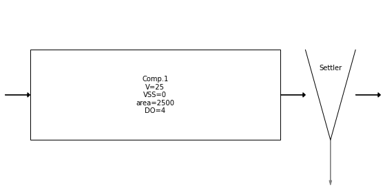
Step 2: Set up the reactor

We will assume a completely stirred tank reactor, thus we will only use one compartment in the reactor model. I will use a volume of 25 m\(^{3}\), which will result in a hydraulic residence time of 6 hours. I will set the biofilm area to 2500 m\(^{2}\), which corresponds to a specific biofilm area of 100 m\(^{2}\)/m:math:^{3}. The maximum biofilm thickness (Lmax) is set to 400 \(\mu\)m and the diffusion boundary layer between the bulk liquid and the biofilm (DBL) is set to 10 \(\mu\)m .

Since it is a pure biofilm reactor, I set VSS=0.

I specify a bulk liquid dissolved oxygen concentration (DO) of 4 g/m\(^{3}\).

The influent is specified as the variable influent we defined above.

After these lines of code, the reactor system is saved in the variable r. I can check the reactor system using the method view_process(). I can also check the influent using the method view_influent().

import biops
import numpy as np
r = biops.ifas.Reactor(influent=influent, volume=25, DO=4, VSS=0, area=2500, Lmax=400*10**-6, DBL=10*10**-6)
r.view_process()
r.view_influent()

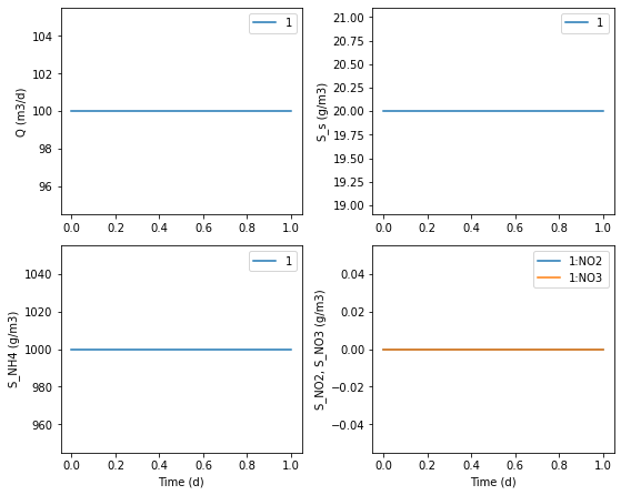
Step 3: Run simulation

Now, we want to investigate how the effluent concentrations and biofilm composition changes over time. Since the influent flow and concentrations are constant, we expect that the effluent and biomass will eventually reach steady state conditions.

The following code will dynamically plot the concentrations of COD and nitrogen. Note that biofilm simulations will take longer time to run than simulations with only suspended growth.

%matplotlib notebook
import matplotlib.pyplot as plt
import time

#Here we set up a multi-panel figure to plot COD, total nitrogen (TN), individual nitrogen species, and biomass composition
plt.rcParams.update({'font.size':10}) #Defines fontsize to use for the axes in the figure
fig, ax = plt.subplots(nrows=2, ncols=2, figsize=(20/2.54, 13/2.54)) #Defines number of panels and figure size
ax[0, 0].set_title('COD (g/m3)', fontsize=10)
ax[0, 1].set_title('TN (g/m3)', fontsize=10)
ax[1, 0].set_title('NH4 (g/m3)', fontsize=10)
ax[1, 1].set_title('NO2(red), NO3(blue) (g/m3)', fontsize=10)
ax[1, 0].set_xlabel('Time (d)')
ax[1, 1].set_xlabel('Time (d)')

fig.tight_layout()

#Here we run a loop for 60 time steps. The default setting is that each time step is one day, so this corresponds to about two monthsge
for i in range(60):
    r.calculate() #This runs the calculation for one time step

    #In the first panel we plot influent and effluent COD concentrations
    ax[0, 0].plot(r.bulklogger['1']['Conc'].index, r.bulklogger['1']['Conc']['S_s'], color='grey')

    #In the second panel we plot influent and effluent TN concentrations
    ax[0, 1].plot(r.bulklogger['1']['Conc'].index, r.bulklogger['1']['Conc'][['S_NH4', 'S_NO2', 'S_NO3']].sum(axis=1), color='grey')

    #In the third panel we plot individual N species in the effluent
    ax[1, 0].plot(r.bulklogger['1']['Conc'].index, r.bulklogger['1']['Conc']['S_NH4'], color='grey')

    #In the fourth panel we plot individual N species in the effluent
    ax[1, 1].plot(r.bulklogger['1']['Conc'].index, r.bulklogger['1']['Conc']['S_NO2'], color='red')
    ax[1, 1].plot(r.bulklogger['1']['Conc'].index, r.bulklogger['1']['Conc']['S_NO3'], color='blue')

    fig.canvas.draw()
    time.sleep(0.05) #This is to slow down the calculations a bit so we can see the figure dynamically updating

Step 4: Explore the biofilm profiles

In the plots above, we see the concentrations in the effluent from the reactor. To find what happened inside the biofilm we can have a look at the information stored in r.biofilmlogger. Data is stored at each time point. I will first check which time points we have available.

print(sorted(r.biofilmlogger['1']['Conc'].keys()))

[0, 1.0, 2.0, 3.0, 4.0, 5.0, 6.0, 7.0, 8.0, 9.0, 10.0, 11.0, 12.0, 13.0, 14.0, 15.0, 16.0, 17.0, 18.0, 19.0, 20.0, 21.0, 22.0, 23.0, 24.0, 25.0, 26.0, 27.0, 28.0, 29.0, 30.0, 31.0, 32.0, 33.0, 34.0, 35.0, 36.0, 37.0, 38.0, 39.0, 40.0, 41.0, 42.0, 43.0, 44.0, 45.0, 46.0, 47.0, 48.0, 49.0, 50.0, 51.0, 52.0, 53.0, 54.0, 55.0, 56.0, 57.0, 58.0, 59.0, 60.0]

I will plot concentration profiles of substrate and biomass components at two time points: day 20 and day 60.

import matplotlib.pyplot as plt

plt.rcParams.update({'font.size':10}) #Defines fontsize to use for the axes in the figure
fig, ax = plt.subplots(nrows=3, ncols=2, figsize=(20/2.54, 17/2.54)) #Defines number of panels and figure size
ax[0, 0].set_title('DO (g/m3)', fontsize=10)
ax[0, 0].plot(r.biofilmlogger['1']['Conc'][20.0]['thickness']*10**6, r.biofilmlogger['1']['Conc'][20.0]['S_O2'], color='blue', label='Day 20')
ax[0, 0].plot(r.biofilmlogger['1']['Conc'][60.0]['thickness']*10**6, r.biofilmlogger['1']['Conc'][60.0]['S_O2'], color='red', label='Day 60')
ax[0, 0].legend()

ax[0, 1].set_title('NH4 (g/m3)', fontsize=10)
ax[0, 1].plot(r.biofilmlogger['1']['Conc'][20.0]['thickness']*10**6, r.biofilmlogger['1']['Conc'][20.0]['S_NH4'], color='blue', label='Day 20')
ax[0, 1].plot(r.biofilmlogger['1']['Conc'][60.0]['thickness']*10**6, r.biofilmlogger['1']['Conc'][60.0]['S_NH4'], color='red', label='Day 60')
ax[0, 1].legend()

ax[1, 0].set_title('NO2 (g/m3)', fontsize=10)
ax[1, 0].plot(r.biofilmlogger['1']['Conc'][20.0]['thickness']*10**6, r.biofilmlogger['1']['Conc'][20.0]['S_NO2'], color='blue', label='Day 20')
ax[1, 0].plot(r.biofilmlogger['1']['Conc'][60.0]['thickness']*10**6, r.biofilmlogger['1']['Conc'][60.0]['S_NO2'], color='red', label='Day 60')
ax[1, 0].legend()

ax[1, 1].set_title('NO3 (g/m3)', fontsize=10)
ax[1, 1].plot(r.biofilmlogger['1']['Conc'][20.0]['thickness']*10**6, r.biofilmlogger['1']['Conc'][20.0]['S_NO3'], color='blue', label='Day 20')
ax[1, 1].plot(r.biofilmlogger['1']['Conc'][60.0]['thickness']*10**6, r.biofilmlogger['1']['Conc'][60.0]['S_NO3'], color='red', label='Day 60')
ax[1, 1].legend()

ax[2, 0].set_title('Biomass (day 20)', fontsize=10)
ax[2, 0].plot(r.biofilmlogger['1']['Conc'][20.0]['thickness'][:-1]*10**6, r.biofilmlogger['1']['Conc'][20.0]['X_OHO'][:-1], color='blue', label='OHO')
ax[2, 0].plot(r.biofilmlogger['1']['Conc'][20.0]['thickness'][:-1]*10**6, r.biofilmlogger['1']['Conc'][20.0]['X_AOB'][:-1], color='red', label='AOB')
ax[2, 0].plot(r.biofilmlogger['1']['Conc'][20.0]['thickness'][:-1]*10**6, r.biofilmlogger['1']['Conc'][20.0]['X_NOB'][:-1], color='magenta', label='NOB')
ax[2, 0].plot(r.biofilmlogger['1']['Conc'][20.0]['thickness'][:-1]*10**6, r.biofilmlogger['1']['Conc'][20.0]['X_AMX'][:-1], color='green', label='Anammox')
ax[2, 0].plot(r.biofilmlogger['1']['Conc'][20.0]['thickness'][:-1]*10**6, r.biofilmlogger['1']['Conc'][20.0]['X_CMX'][:-1], color='orange', label='Comammox')
ax[2, 0].plot(r.biofilmlogger['1']['Conc'][20.0]['thickness'][:-1]*10**6, r.biofilmlogger['1']['Conc'][20.0]['X_I'][:-1], color='grey', label='Inert')

ax[2, 1].set_title('Biomass (day 60)', fontsize=10)
ax[2, 1].plot(r.biofilmlogger['1']['Conc'][60.0]['thickness'][:-1]*10**6, r.biofilmlogger['1']['Conc'][60.0]['X_OHO'][:-1], color='blue', label='OHO')
ax[2, 1].plot(r.biofilmlogger['1']['Conc'][60.0]['thickness'][:-1]*10**6, r.biofilmlogger['1']['Conc'][60.0]['X_AOB'][:-1], color='red', label='AOB')
ax[2, 1].plot(r.biofilmlogger['1']['Conc'][60.0]['thickness'][:-1]*10**6, r.biofilmlogger['1']['Conc'][60.0]['X_NOB'][:-1], color='magenta', label='NOB')
ax[2, 1].plot(r.biofilmlogger['1']['Conc'][60.0]['thickness'][:-1]*10**6, r.biofilmlogger['1']['Conc'][60.0]['X_AMX'][:-1], color='green', label='Anammox')
ax[2, 1].plot(r.biofilmlogger['1']['Conc'][60.0]['thickness'][:-1]*10**6, r.biofilmlogger['1']['Conc'][60.0]['X_CMX'][:-1], color='orange', label='Comammox')
ax[2, 1].plot(r.biofilmlogger['1']['Conc'][60.0]['thickness'][:-1]*10**6, r.biofilmlogger['1']['Conc'][60.0]['X_I'][:-1], color='grey', label='Inert')
ax[2, 1].legend(bbox_to_anchor=(1,1))

ax[2, 0].set_xlabel('Thickness (um)')
ax[2, 1].set_xlabel('Thickness (um)')
fig.tight_layout()

We see that the biofilm has grown to its maximum allowed thickness, 400 \(\mu\)m. At day 20, AOB are dominating the biofilm, we have a lot of nitrite in the water, and dissolved oxygen is completely consumed at a biofilm thickness of about 200 \(\mu\)m. At day 60, there is a balance between AOB and NOB and both ammonium and nitrite are almost completely removed from the bulk liquid. The amount of inert material in the biofilm has increased.